大模型Attention发展历程

MHA Multi Head Attention

MHA 相比于传统的 Self-Attention 提升了模型的表达能力。例如一个专家组对比一个专家。
先看代码：

def forward(
        self,
        hidden_states: torch.Tensor,
        position_embeddings: tuple[torch.Tensor, torch.Tensor],
        attention_mask: Optional[torch.Tensor],
        past_key_values: Optional[Cache] = None,
        cache_position: Optional[torch.LongTensor] = None,
        **kwargs: Unpack[TransformersKwargs],
    ) -> tuple[torch.Tensor, torch.Tensor]:
    input_shape = hidden_states.shape[:-1]
    hidden_shape = (*input_shape, -1, self.head_dim)

    query_states = self.q_proj(hidden_states).view(hidden_shape).transpose(1, 2)
    key_states = self.k_proj(hidden_states).view(hidden_shape).transpose(1, 2)
    value_states = self.v_proj(hidden_states).view(hidden_shape).transpose(1, 2)

    cos, sin = position_embeddings
    query_states, key_states = apply_rotary_pos_emb(query_states, key_states, cos, sin)

    attn_output, attn_weights = attention_interface(
        self,
        query_states,
        key_states,
        value_states,
        attention_mask,
        dropout=0.0 if not self.training else self.attention_dropout,
        scaling=self.scaling,
        **kwargs,
    )

    attn_output = attn_output.reshape(*input_shape, -1).contiguous()
    attn_output = self.o_proj(attn_output)
    return attn_output, attn_weights

这个 attention 是 Multi-head self-attention，注意力有头这个概念。其中，Q K V 这三个向量分别是由 hidden_states 乘上一个 Linear 层来计算的。这里面由于是多头注意力机制，所以需要让 Q K V 的 shape 变为 (batch, seq_len, num_head, head_dim)。之后 transpose 成 (batch, num_head, seq_len, head_dim)，这么做的目的是为了让后续计算时，每个头可以独立进行注意力计算，让 num_head 变为“批次”的一部分，注意力仅在 seq_len 维度计算，而不把不同的 head 混在一起算。
再算完这几个向量后，需要对 Q K 向量添加位置信息，这就是 apply_rotary_pos_emb 的作用。之后就是 attention 的计算，也就是我们说的公式:

\begin{aligned} \text{Attention}(Q, K, V) &= \text{softmax}\left(\frac{QK^T}{\sqrt{d_k}}\right)V \end{aligned}

其中，QK 的意思是 Q 和 K 的点积，表示 Q 和 K 之间的相似性，更进一步，这个向量是词向量，是词在高维空间的数值映射。词向量之间相关度高表示什么？是不是在一定程度上（不是完全）表示，在关注词 A 的时候，应当给予词 B 更多的关注？除以 $\sqrt{d_k}$ 的作用是训练时防止梯度消失。
算完 attention 后，再被 o_projection 映射，结果就算出来了。

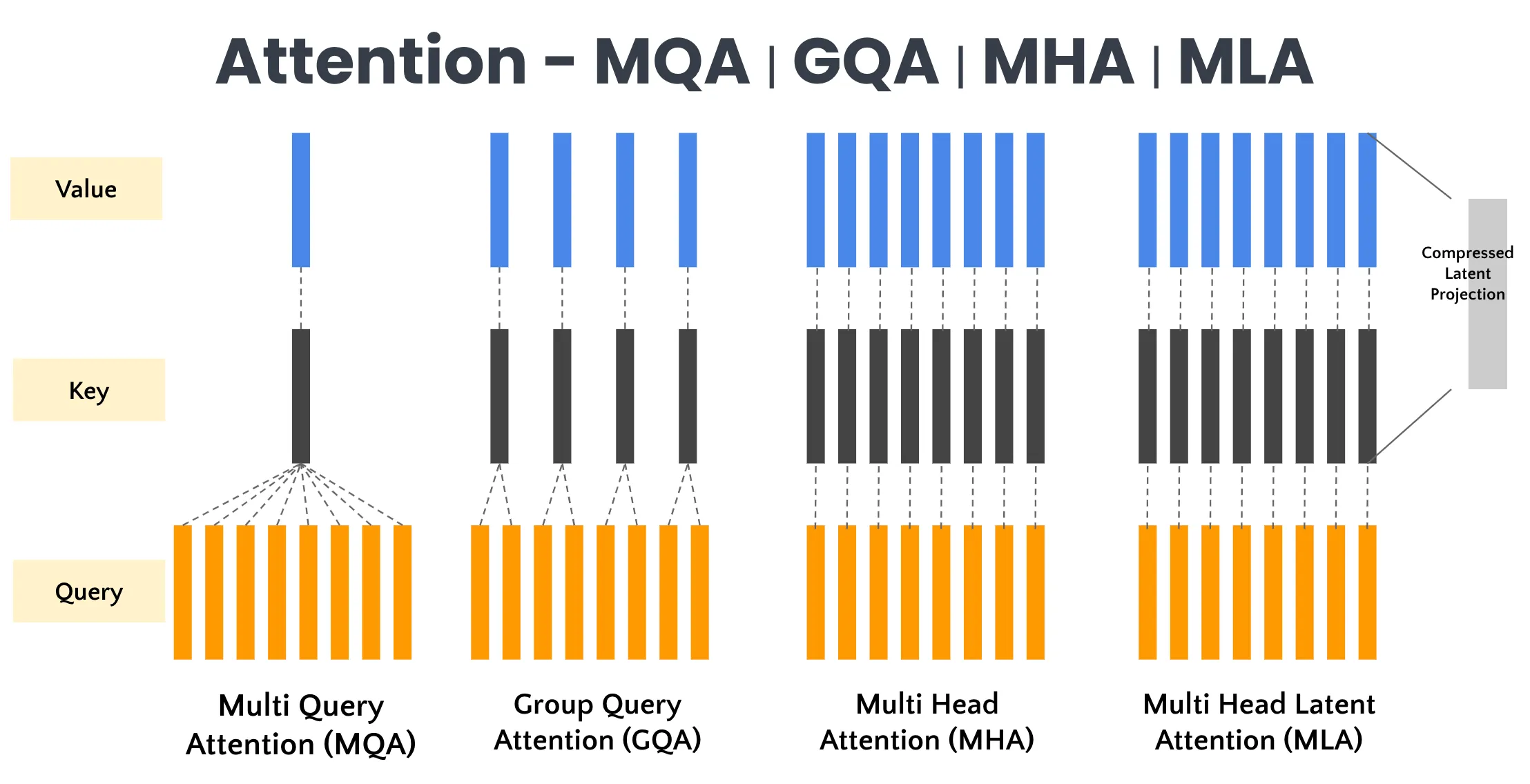
MHA (Multi-Head Attention)：假设头个数为32，
- 配置：每个 Query 头都有自己独立的 Key 头和 Value 头。
- 数量：32 个 Q 头，对应 32 个 K 头和 32 个 V 头。
- 特点：完全独立，信息隔离性好，模型表达能力强。
  总结：MHA 多头自注意力机制是效果最好的也是最慢的，而 MQA 和 GQA 则是通过不同的方式来提升计算效率。
  一些比较出名的模型，如 LLama2-7B、LLama2-13B 使用的都是这种架构。

MQA Multi Query Attention

相比 MHA，MQA 允许一个 Query 头同时关注多个 Key 头和 Value 头，从而在保证信息隔离性的前提下，提升模型的计算效率。

MQA (Multi-Query Attention)：假设头个数为32，
- 配置：所有的 Query 头共享同一组 Key 和 Value 头。
- 数量：32 个 Q 头，对应 1 个 K 头和 1 个 V 头。
- 特点：极端压缩，推理速度极快，但模型效果下降明显（因为所有头被迫看同样的 K/V 信息）。
  目前没听说哪个模型全程使用这个架构。但是 DeepSeek V3.2 的 decode 阶段使用了该方式。

GQA Group Query Attention

GQA 相比 MHA，其主要区别在于，GQA 是先进行“组内”注意力计算，再进行“组间”注意力计算。也就是说，GQA 首先将 Q K V 分成多组，然后在组内进行注意力计算，最后在组间进行注意力计算。推理速度更快，普遍用于 70B 及更大的模型中。MHA 则用于稍微小一点的模型中。

def forward(
        self,
        hidden_states: torch.Tensor,
        attention_mask: Optional[torch.Tensor] = None,
        position_ids: Optional[torch.LongTensor] = None,
        past_key_values: Optional[Cache] = None,
        output_attentions: bool = False,
        use_cache: bool = False,
        cache_position: Optional[torch.LongTensor] = None,
        position_embeddings: Optional[tuple[torch.Tensor, torch.Tensor]] = None,  # necessary, but kept here for BC
    ) -> tuple[torch.Tensor, Optional[torch.Tensor], Optional[tuple[torch.Tensor]]]:
    bsz, q_len, _ = hidden_states.size()

    query_states = self.q_proj(hidden_states)
    key_states = self.k_proj(hidden_states)
    value_states = self.v_proj(hidden_states)

    query_states = query_states.view(bsz, q_len, -1, self.head_dim).transpose(1, 2)
    key_states = key_states.view(bsz, q_len, -1, self.head_dim).transpose(1, 2)
    value_states = value_states.view(bsz, q_len, -1, self.head_dim).transpose(1, 2)

    cos, sin = position_embeddings
    query_states, key_states = apply_rotary_pos_emb(query_states, key_states, cos, sin, position_ids)

    # repeat k/v heads if n_kv_heads < n_heads
    key_states = repeat_kv(key_states, self.num_key_value_groups)
    value_states = repeat_kv(value_states, self.num_key_value_groups)

    attn_weights = torch.matmul(query_states, key_states.transpose(2, 3)) / math.sqrt(self.head_dim)

    if attention_mask is not None:  # no matter the length, we just slice it
        causal_mask = attention_mask[:, :, :, : key_states.shape[-2]]
        attn_weights = attn_weights + causal_mask

    # upcast attention to fp32
    attn_weights = nn.functional.softmax(attn_weights, dim=-1, dtype=torch.float32).to(query_states.dtype)
    attn_weights = nn.functional.dropout(attn_weights, p=self.attention_dropout, training=self.training)
    attn_output = torch.matmul(attn_weights, value_states)

    if attn_output.size() != (bsz, self.num_heads, q_len, self.head_dim):
        raise ValueError(
            f"`attn_output` should be of size {(bsz, self.num_heads, q_len, self.head_dim)}, but is"
            f" {attn_output.size()}"
        )

    attn_output = attn_output.transpose(1, 2).contiguous()
    attn_output = attn_output.reshape(bsz, q_len, self.hidden_size)

    attn_output = self.o_proj(attn_output)

    if not output_attentions:
        attn_weights = None

    return attn_output, attn_weights

可以看见代码里有一个 repeat_kv 的操作，作用是将较少的 Key/Value 头复制扩展，使它们能和 Query 的头数一一对应进行矩阵乘法。这正是 GQA 的典型操作：“分组共享，通过复制来对齐”。

GQA (Grouped Query Attention)：
- 配置：将 Query 头分组，每组 Query 头共享一组 Key 和 Value。
- 数量：例如分为 8 组（Group=8）。32 个 Q 头，对应 8 个 K 头和 8 个 V 头（每4个Q头共享1个K/V头）。
- 特点：介于 MHA 和 MQA 之间。比 MQA 效果好（保留了部分独立性），比 MHA 速度快（KV Cache 大小减少了 4 倍）。
  GQA 相比于 MHA，效果上几乎相近，而速度却能达到 MQA 的水平，被广泛的应用在现在的大模型上。
  LLama2-70B、LLama3、Qwen2 全系列使用的都是这种架构。

MLA Multi Latent Attention

def forward(
        self,
        hidden_states: torch.Tensor,
        position_embeddings: tuple[torch.Tensor, torch.Tensor],
        attention_mask: Optional[torch.Tensor],
        past_key_values: Optional[Cache] = None,
        cache_position: Optional[torch.LongTensor] = None,
        **kwargs: Unpack[FlashAttentionKwargs],
    ) -> tuple[torch.Tensor, Optional[torch.Tensor], Optional[tuple[torch.Tensor]]]:
    batch_size, seq_length = hidden_states.shape[:-1]
    query_shape = (batch_size, seq_length, -1, self.qk_head_dim)
    key_shape = (batch_size, seq_length, -1, self.qk_nope_head_dim + self.v_head_dim)

    if self.q_lora_rank is None:
        q_states = self.q_proj(hidden_states)
    else:
        q_states = self.q_b_proj(self.q_a_layernorm(self.q_a_proj(hidden_states)))
    q_states = q_states.view(query_shape).transpose(1, 2)
    q_pass, q_rot = torch.split(q_states, [self.qk_nope_head_dim, self.qk_rope_head_dim], dim=-1)

    compressed_kv = self.kv_a_proj_with_mqa(hidden_states)
    k_pass, k_rot = torch.split(compressed_kv, [self.kv_lora_rank, self.qk_rope_head_dim], dim=-1)

    k_pass = self.kv_b_proj(self.kv_a_layernorm(k_pass)).view(key_shape).transpose(1, 2)
    k_pass, value_states = torch.split(k_pass, [self.qk_nope_head_dim, self.v_head_dim], dim=-1)

    k_rot = k_rot.view(batch_size, 1, seq_length, self.qk_rope_head_dim)

    cos, sin = position_embeddings
    if self.config.rope_interleave:  # support using interleaved weights for efficiency
        q_rot, k_rot = apply_rotary_pos_emb_interleave(q_rot, k_rot, cos, sin)
    else:
        q_rot, k_rot = apply_rotary_pos_emb(q_rot, k_rot, cos, sin)
    k_rot = k_rot.expand(*k_pass.shape[:-1], -1)

    query_states = torch.cat((q_pass, q_rot), dim=-1)
    key_states = torch.cat((k_pass, k_rot), dim=-1)

    if past_key_values is not None:
        # sin and cos are specific to RoPE models; cache_position needed for the static cache
        cache_kwargs = {"sin": sin, "cos": cos, "cache_position": cache_position}
        key_states, value_states = past_key_values.update(key_states, value_states, self.layer_idx, cache_kwargs)

    if self.config._attn_implementation == "flash_attention_2" and self.qk_head_dim != self.v_head_dim:
        value_states = F.pad(value_states, [0, self.qk_head_dim - self.v_head_dim])

    attention_interface: Callable = eager_attention_forward
    if self.config._attn_implementation != "eager":
        attention_interface = ALL_ATTENTION_FUNCTIONS[self.config._attn_implementation]

    attn_output, attn_weights = attention_interface(
        self,
        query_states,
        key_states,
        value_states,
        attention_mask,
        dropout=0.0 if not self.training else self.attention_dropout,
        scaling=self.scaling,
        **kwargs,
    )

    if self.config._attn_implementation == "flash_attention_2" and self.qk_head_dim != self.v_head_dim:
        attn_output = attn_output[:, :, :, : self.v_head_dim]

    attn_output = attn_output.reshape(batch_size, seq_length, -1).contiguous()
    attn_output = self.o_proj(attn_output)
    return attn_output, attn_weights

上面代码是 MLA 的流程。可以分为以下几步：

Query 的生成与压缩
DeepSeek 对 Q 进行了压缩，减少计算量

# 这一部分对应 Query 的生成
if self.q_lora_rank is None:
    # 如果没有设置压缩秩，则使用标准投影
    q_states = self.q_proj(hidden_states)
else:
    # 【核心 MLA 特征】：Query 低秩压缩
    # 1. q_a_proj: 降维 (hidden -> low_rank)
    # 2. q_a_layernorm: 训练时加了个layernorm，防止梯度爆炸，归一化
    # 3. q_b_proj: 升维 (low_rank -> num_heads * qk_head_dim)
    q_states = self.q_b_proj(self.q_a_layernorm(self.q_a_proj(hidden_states)))

q_states = q_states.view(query_shape).transpose(1, 2)

# 【核心 MLA 特征】：解耦 RoPE
# 将 Query 分割为两部分：一部分不带位置信息，一部分带位置信息
q_pass, q_rot = torch.split(q_states, [self.qk_nope_head_dim, self.qk_rope_head_dim], dim=-1)

KV 的压缩与潜在向量生成

# 【核心 MLA 特征】：KV 压缩
# 将输入投影到一个非常小的压缩向量 (Latent Vector)
# 这就是推理时缓存的 "KV Cache"，体积非常小！
compressed_kv = self.kv_a_proj_with_mqa(hidden_states)

# 将压缩向量拆分：
# k_pass: 压缩后的 KV 内容特征 (用于后续还原)
# k_rot: 专门用于位置编码的部分
k_pass, k_rot = torch.split(compressed_kv, [self.kv_lora_rank, self.qk_rope_head_dim], dim=-1)

KV 的解压与还原

# 1. 对压缩的内容特征进行 LayerNorm
# 2. kv_b_proj: 升维投影，将低维 Latent 还原成高维的 Key 和 Value
k_pass = self.kv_b_proj(self.kv_a_layernorm(k_pass)).view(key_shape).transpose(1, 2)

# 分离还原后的 Key 和 Value
k_pass, value_states = torch.split(k_pass, [self.qk_nope_head_dim, self.v_head_dim], dim=-1)

虽然我们在 Cache 里存的是压缩后的向量，但在计算当前时刻的 Attention 分数时，需要将其还原成完整的多头 Key 和 Value。虽然计算量增加了一些，但换来了显存带宽的大幅节省。

位置编码与拼接

# 对专门的位置部分应用 RoPE
cos, sin = position_embeddings
q_rot, k_rot = apply_rotary_pos_emb(q_rot, k_rot, cos, sin)

# 扩展 k_rot 维度以匹配多头

# 【核心 MLA 特征】：重组
# 将内容部分 和位置部分 拼接
query_states = torch.cat((q_pass, q_rot), dim=-1)
key_states = torch.cat((k_pass, k_rot), dim=-1)

最终参与计算的 query_states 和 key_states 是由“非旋转部分”和“旋转部分”拼接而成的。这样做的好处是，位置信息不会破坏压缩向量的低秩结构。为什么位置编码要这么做呢？因为在实现 MLA 的时候，有一个小技巧叫做“矩阵吸收”。

x W_{down}^Q W_{up,i}^Q (W_{up,i}^K{})^T (c^{KV}{})^T

在这个公式中，可以将 kv 的上投影矩阵 $W_{up,i}^K$ 看成是 $W_{up,i}^Q$ ，这样子，位置信息部分就可以通过矩阵吸收的方式，被 $W_{down}^Q$ “吸收”进去了。但是如果加了常规旋转位置编码的话，位置信息部分就无法被 $W_{down}^Q$ “吸收”进去了。可以看见被隔断了。无法吸收，会导致推理效率下降。

x W_{down}^Q W_{up,i}^Q R_{m} R_{n}^T (W_{up,i}^K{})^T (c^{KV}{})^T

所以引入了 Decoupled RoPE (解耦 RoPE)。q_rot 和 k_rot 分开处理，这样位置编码和内容编码就可以分开处理，互不干扰。

注意力计算

# 更新 KV Cache (这里存储的通常是还原后的 K 和 V，或者是压缩向量，取决于具体的 Cache 实现)
if past_key_values is not None:
    key_states, value_states = past_key_values.update(...)

# 【Flash Attention 兼容性处理】
# 如果 QK 的维度和 V 的维度不一样，需要 Padding 对齐
if self.config._attn_implementation == "flash_attention_2" and self.qk_head_dim != self.v_head_dim:
    value_states = F.pad(value_states, [0, self.qk_head_dim - self.v_head_dim])

# 调用标准注意力接口计算
attn_output, attn_weights = attention_interface(...)

# 去除 Padding
if ...:
    attn_output = attn_output[:, :, :, : self.v_head_dim]

# 输出投影
attn_output = self.o_proj(attn_output)

MLA (Multi-Head Latent Attention)
- 配置：通过生成 compressed_kv，将 KV Cache 的大小压缩了 90% 以上。存储上 compressed_kv 只有一份，接近 MQA。
- 数量：通过 kv_b_proj 动态还原 KV，保留了多头注意力的表达能力。每个头一个 KV 数量，这一部分接近 MHA。
- 特点：通过 split 和 cat 操作，把位置信息和内容信息分开处理，使得压缩机制能与 RoPE 完美兼容。

NSA Natural Sparse Attention

该注意力机制首次被提出是在 2025 年的 2 月。由 DeepSeek 针对长序列处理提出的原生稀疏注意力机制，属于 block-wise 的稀疏方案。这个目前只存在于论文中，没有实际用于某个模型。直到 Deepseek-V3.2 中，他们提出了 DSA，可以说是 NSA 的一个变种实现，属于 token-wise 的稀疏方案。

压缩块，计算块间注意力
标准自注意力需要计算序列中每个词元（Token）与其他所有词元的关系。对于一个长度为 N 的序列，需要计算 N*N 个注意力权重，随长度二次增长。
解决方案是，NSA 不再以单个 token 为基本计算单元，而是将连续的多个 token 聚合成一个 block。例如，将 4096 个词元的序列划分为 64 个块，每个块包含 64 个 token。
计算流程转变：
之前（标准注意力）：处理 4096 个 token -> 需要处理 4096 * 4096≈16.7M 个关系对。
之后（块压缩）：处理 64 个 block -> 先计算块与块之间的注意力。此时，需要处理的关系对数量骤降至 64 * 64=4096 个。
重要性筛选：选出重要的 K 个块
在压缩后的 block 中，筛选出需要详细看的部分：
块压缩是假设所有 block 都同等重要。但实际上，对于当前要处理的 token 来说，某些 block 是关键的而其他的是次要的。NSA 引入动态机制，根据当前的 Q 内容，评估并筛选出最相关的少量关键 block。
系统会为每个 block 计算一个“重要性分数”。这个分数通常基于当前 Q 与每个 block 的“摘要向量”（通常是 block 内 token 的均值或通过一个小型网络生成）的相似度。
在块压缩的基础上增加重要性筛选，系统从64个块中选出最相关的 K 个块（例如 K=8），额外计算当前查询向量与这 K 个关键块内全部 token 的注意力。
滑动窗口
为了保证局部上下文信息的完整性，token 不但要关注遥远的关键块，还要关注紧挨着它的其他 token。NSA 强制性地规定，无论重要性筛选的结果如何，每个 token 都必须关注以其自身为中心的一个局部窗口内的所有其他token。这个窗口是“滑动”的，因为它随着 token 位置的变化而移动。例如，假设滑动窗口大小为 256。那么对于序列中第 500 个 token，无论如何它都会关注第 500-255 至第 500 这个范围内的所有 token。

DSA DeepSeek Sparse Attention

DSA 首次被应用在 Deepseek V3.2 Exp 中，属于 token-wise 的稀疏方案。DeepSeek-V3.2-Exp 仅在 DeepSeek-V3 的基础上新增了 Lightning Indexer 模块，用于选择参与 attention 的 token。
该模块的主要输入是 compressed_q 与 MLA 的输入矩阵 hidden_states，输出则是每个 token 所对应的 2048 个可参与 attention 计算的历史 token 的 index。
被选中的 2048 个 token 会在 attention 的 mask 阶段发挥作用：通过将未选中的位置的 mask 值设为 inf，在经过 softmax 之后，就能有效去除不需要参与 attention 的 token。这样实现了高效的稀疏化，显著降低了计算量。从O(L^2)降到了O(LK)，其中 K<<L 为 2048。
Indexer 代码（来自于官方 DeepSeek V3.2 仓库）：

def fp8_index(
    q: torch.Tensor,
    q_s: torch.Tensor,
    k: torch.Tensor,
    k_s: torch.Tensor,
) -> torch.Tensor:
    """
    Perform index score using FP8 precision.

    Args:
        q (torch.Tensor): The Q tensor, must be contiguous.
        q_s (torch.Tensor): The scaling factor for Q (float), must be contiguous.
        k (torch.Tensor): The K tensor, must be contiguous.
        k_s (torch.Tensor): The scaling factor for K (e8m0 here), must be contiguous.

        fp8 q @ fp8 k -> fp32 logits
        relu(fp32 logits) * q_s (weights) -> fp32 logits
        fp32 logits -> fp32 logits_sum
        fp32 logits_sum * k_s (e8m0) -> fp32 index_score
    """
    return fp8_index_kernel(q.shape[2], q.shape[3])(q, q_s, k, k_s)

class Indexer(torch.nn.Module):
    def __init__(self, args: ModelArgs):
        super().__init__()
        self.dim: int = args.dim
        self.n_heads: int = args.index_n_heads
        self.n_local_heads = args.index_n_heads // world_size
        self.head_dim: int = args.index_head_dim
        self.rope_head_dim: int = args.qk_rope_head_dim
        self.index_topk: int = args.index_topk
        self.q_lora_rank: int = args.q_lora_rank
        self.wq_b = Linear(self.q_lora_rank, self.n_heads * self.head_dim)
        self.wk = Linear(self.dim, self.head_dim)
        self.k_norm = LayerNorm(self.head_dim)
        # weights_proj in the checkpoint is stored in bf16, while the parameters here are stored in fp32 for convenient.
        self.weights_proj = Linear(self.dim, self.n_heads, dtype=torch.float32)
        self.softmax_scale = self.head_dim ** -0.5
        self.scale_fmt = args.scale_fmt

        self.register_buffer("k_cache", torch.zeros(args.max_batch_size, args.max_seq_len, self.head_dim, dtype=torch.float8_e4m3fn), persistent=False)
        self.register_buffer("k_scale_cache", torch.zeros(args.max_batch_size, args.max_seq_len, self.head_dim // block_size, dtype=torch.float32), persistent=False)

    def forward(self, x: torch.Tensor, qr: torch.Tensor, start_pos: int, freqs_cis: torch.Tensor, mask: Optional[torch.Tensor]):
        bsz, seqlen, _ = x.size()
        end_pos = start_pos + seqlen
        q = self.wq_b(qr)
        q = q.view(bsz, seqlen, self.n_heads, self.head_dim)
        q_pe, q_nope = torch.split(q, [self.rope_head_dim, self.head_dim - self.rope_head_dim], dim=-1)
        # rope in indexer is not interleaved
        q_pe = apply_rotary_emb(q_pe, freqs_cis, False)
        q = torch.cat([q_pe, q_nope], dim=-1)
        k = self.wk(x)
        k = self.k_norm(k)
        k_pe, k_nope = torch.split(k, [self.rope_head_dim, self.head_dim - self.rope_head_dim], dim=-1)
        # rope in indexer is not interleaved
        k_pe = apply_rotary_emb(k_pe.unsqueeze(2), freqs_cis, False).squeeze(2)
        k = torch.cat([k_pe, k_nope], dim=-1)
        q = rotate_activation(q)
        k = rotate_activation(k)
        q_fp8, q_scale = act_quant(q, block_size, self.scale_fmt)
        k_fp8, k_scale = act_quant(k, block_size, self.scale_fmt)
        self.k_cache[:bsz, start_pos:end_pos] = k_fp8
        self.k_scale_cache[:bsz, start_pos:end_pos] = k_scale
        weights = self.weights_proj(x.float()) * self.n_heads ** -0.5
        weights = weights.unsqueeze(-1) * q_scale * self.softmax_scale
        index_score = fp8_index(q_fp8.contiguous(), weights, self.k_cache[:bsz, :end_pos].contiguous(), self.k_scale_cache[:bsz, :end_pos].contiguous())
        if mask is not None:
            index_score += mask
        topk_indices = index_score.topk(min(self.index_topk, end_pos), dim=-1)[1]
        topk_indices_ = topk_indices.clone()
        dist.broadcast(topk_indices_, src=0)
        assert torch.all(topk_indices == topk_indices_), f"{topk_indices=} {topk_indices_=}"
        return topk_indices

公式如下：

I_{t,s} = \sum_{j=1}^{H_{I}} w_{t,j}^{I} \cdot \operatorname{ReLU}\left( \boldsymbol{q}_{t,j}^{I} \cdot \boldsymbol{k}_{s}^{I} \right)

总体框架如下：

其中，绿色部分是 indexer 实现。而框住的部分是函数 fp8_index 部分。可以看到，虽然说 attention 的计算复杂度降低了，但是实际上选择不同 token 重要性这个 indexer 模块，也算是个 attention。还是需要计算查询相对于之前每个 token 的 attention 的重要性分数，复杂度还是 $O(n^2)$ 。只不过这个过程是在 fp8 精度下进行的，所以效率会比较高。

为什么需要哈达玛变换"rotate_activation"？
直接量化 q 和 k 向量可能会造成精度损失。引入旋转变换操作：将大范围数值打散到小范围。可以与随机的正交矩阵相乘来做这件事，使得向量数值分布均匀且模长不变。不过矩阵乘法代价较大。于是使用小代价的哈达玛变换。

最后得出的topk_indices，会作为 mask 输入到 MLA 中，从而实现稀疏化。可以看下面代码。
对于 Deepseek V3.2 的 attention 实现而言：

def forward(self, x: torch.Tensor, start_pos: int, freqs_cis: torch.Tensor, mask: Optional[torch.Tensor]):
    """
    Forward pass for the Multi-Head Latent Attention (MLA) Layer.

    Args:
        x (torch.Tensor): Input tensor of shape (batch_size, seq_len, dim).
        start_pos (int): Starting position in the sequence for caching.
        freqs_cis (torch.Tensor): Precomputed complex exponential values for rotary embeddings.
        mask (Optional[torch.Tensor]): Mask tensor to exclude certain positions from attention.

    Returns:
        torch.Tensor: Output tensor with the same shape as the input.
    """
    bsz, seqlen, _ = x.size()
    end_pos = start_pos + seqlen
    qr = self.q_norm(self.wq_a(x))
    q = self.wq_b(qr)
    q = q.view(bsz, seqlen, self.n_local_heads, self.qk_head_dim)
    q_nope, q_pe = torch.split(q, [self.qk_nope_head_dim, self.qk_rope_head_dim], dim=-1)
    q_pe = apply_rotary_emb(q_pe, freqs_cis)
    kv = self.wkv_a(x)
    kv, k_pe = torch.split(kv, [self.kv_lora_rank, self.qk_rope_head_dim], dim=-1)
    kv = self.kv_norm(kv)
    k_pe = apply_rotary_emb(k_pe.unsqueeze(2), freqs_cis)
    # we use fp8 kv cache in actual deployment, so here we simulate the precision by casting kv to fp8 and then back to bf16.
    kv_fp8, kv_scale = act_quant(kv, block_size, self.scale_fmt)
    kv = (kv_fp8.view(-1, block_size).float() * kv_scale.view(-1, 1)).to(kv.dtype).view_as(kv)
    self.kv_cache[:bsz, start_pos:end_pos] = kv
    self.pe_cache[:bsz, start_pos:end_pos] = k_pe.squeeze(2)
    if mask is not None:    # MHA prefill
        q = torch.cat([q_nope, q_pe], dim=-1)
        kv = self.wkv_b(kv)
        kv = kv.view(bsz, seqlen, self.n_local_heads, self.qk_nope_head_dim + self.v_head_dim)
        k_nope, v = torch.split(kv, [self.qk_nope_head_dim, self.v_head_dim], dim=-1)
        k = torch.cat([k_nope, k_pe.expand(-1, -1, self.n_local_heads, -1)], dim=-1)
        scores = torch.einsum("bshd,bthd->bsht", q, k).mul_(self.softmax_scale)

        # indexer
        topk_indices = self.indexer(x, qr, start_pos, freqs_cis, mask)
        index_mask = torch.full((bsz, seqlen, seqlen), float("-inf"), device=x.device).scatter_(-1, topk_indices, 0)
        index_mask += mask
        scores += index_mask.unsqueeze(2)

        scores = scores.softmax(dim=-1)
        x = torch.einsum("bsht,bthd->bshd", scores, v)
    else:                   # MQA decode
        if self.dequant_wkv_b is None and self.wkv_b.scale is not None:
            self.dequant_wkv_b = weight_dequant(self.wkv_b.weight, self.wkv_b.scale)
        wkv_b = self.wkv_b.weight if self.dequant_wkv_b is None else self.dequant_wkv_b
        wkv_b = wkv_b.view(self.n_local_heads, -1, self.kv_lora_rank)
        q_nope = torch.einsum("bshd,hdc->bshc", q_nope, wkv_b[:, :self.qk_nope_head_dim])
        scores = (torch.einsum("bshc,btc->bsht", q_nope, self.kv_cache[:bsz, :end_pos]) +
                    torch.einsum("bshr,btr->bsht", q_pe, self.pe_cache[:bsz, :end_pos])) * self.softmax_scale

        # indexer
        topk_indices = self.indexer(x, qr, start_pos, freqs_cis, mask)
        index_mask = torch.full((bsz, 1, end_pos), float("-inf"), device=x.device).scatter_(-1, topk_indices, 0)
        scores += index_mask.unsqueeze(2)

        scores = scores.softmax(dim=-1)
        x = torch.einsum("bsht,btc->bshc", scores, self.kv_cache[:bsz, :end_pos])
        x = torch.einsum("bshc,hdc->bshd", x, wkv_b[:, -self.v_head_dim:])
    x = self.wo(x.flatten(2))
    return x

caijizhuo

attention发展历程